---

The Trent Farm Photos Appendix

"On the Possibility that the McMinnville Photos Show a Distant Unidentified Object (UO)"

[NOTE: Click on any of the figure names to view the figure]

(This was written in 1976-1977 - exact date not recorded - but was not included in the previous publication. It is published here for the first time. There have been some clarifying comments added in April, 2000.)

This appendix is provided to supply certain supplemental information that will prove useful in evaluating the analysis presented in the main text, in particular the analysis related to the determination of the amount and effects of veiling glare. The information is provided in a series of figures, each of which is described below . Further information is available from the author.

In the main text the relative brightness of a vertical , white shaded surface was estimated from the image brightness of the shadow on the distant house wall. There has been some question an to whether or not the wall was "truly" white. Therefore I have made another estimate based upon the image brightness of the nearby (Trent) house that appears at the right hand side of photo 2. This house was (according to Mrs. Trent in 1975) painted white only about a year before the pictures were taken. An image of the corner of the house just below the eave appears in the second UO photo at the right hand side. 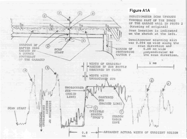(The corresponding image in the first UO photo was cut off the original negative sometime after publication in the Telephone Register newspaper, which shows the corner of the house in both photos.) Figure A1 illustrates the calculation of the brightness of a vertical white surface from the brightness of the image of the western corner of the south wall of the nearby house. Although the veiling glare correction is larger (because it is immediately adjacent to the sky), there is no atmospheric brightening correction. The brightness of a horizontal, shaded white surface based on this nearby house image differs only slightly from the value obtained using the image of the distant house.
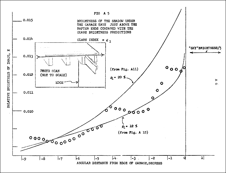
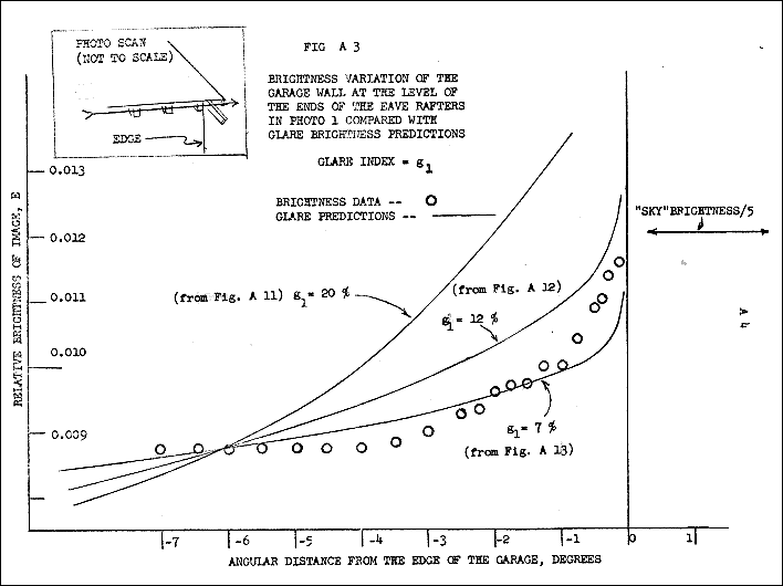
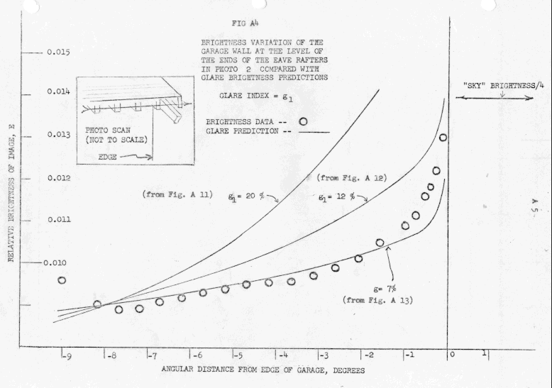
As pointed out in the main text, certain evidence suggests that 12% may be an upper bound on the glare index (defined as the brightness of a perfectly intrinsically black UO image divided by the adjacent sky brightness; see the text and see below). The evidence for this is presented in Figures A3, A4 & A5. These figures contain data on the relative brightnesses of images (garage roof, wall) which, if there were no veiling glare, would have (approximately) constant intrinsic brightness (because of constant reflectivity) over angular distances of at least several degrees away from the object/sky boundary. Figure A2 illustrates the variation of the brightness of the garage roof in each picture. The angular distances are measured along the scan directions indicated by the arrows. Figures A3 and A4 illustrate the brightness variation of the garage wall at the level of the rafter ends, and Fig. A5 illustrates the brightness variation of the shadow that is just under the edge of the roof and Just above the rafter ends. The variation in brightness is mostly caused by veiling glare...light from the adjacent sky is scattered by camera optics into the image of the darker roof or wall.

************************************************************************
FIG. A1

THE SOUTHWEST CORNER OF THE WALL AND EAVE OF THE NEARBY (TRENT) HOUSE APPEARS AT THE RIGHT HAND SIDE OF PHOTO 2. THIS HOUSE WAS REPORTEDLY PAINTED WHITE WITHIN THE YEAR BEFORE THE PICTURES WERE TAKEN.
SINCE THE SUN WAS SLIGHTLY NORTH OF WEST (OR IF IN THE MORNING, SLIGHTLY NORTH OF DUE EAST AT AN ANGULAR ELEVATION OF ABOUT 25 DEGREES), AND SINCE THE ROOF OF THE HOUSE HAD A SMALL EAVE , THE SOUTH WALL WAS SHADED FROM THE DIRECT SUN.
IT WAS, HOWEVER, ILLUMINATED BY SKYLIGHT AND GROUND-REFLECTED LIGHT. THUS THE INTRINSIC BRIGHTNESS OF THE WALL SHOULD BE THE SAME (OR PERHAPS SLIGHTLY GREATER, SINCE THERE WAS NO EAVE SHADING IT) AS THAT OF THE SHADED PART OF THE WALL OF THE DISTANT WHITE HOUSE. FROM THE DENSITY MEASURMENTS AND TRANSFER CURVE:

Ewall image = 0.021 (1/2) degree from the edge

Esky image = 0.065 adjacent to the wall

WHEN THE GLARE INDEX IS 12%, A DARK AREA NEXT TO A UNIFORMLY BRIGHT AREA HAS A GLARE OF ABOUT 6% AT A DISTANCE OF 0.5 degrees INTO THE DARK AREA IMAGE. THE SKY BRIGHTNESS IS NOT UNIFORMLY BRIGHT. NEVERTHELESS, A GOOD APPROXIMATION TO THE INTRINSIC RELATIVE BRIGHTNESS OF THE HOUSE WALL IS

Bvertical,white,shaded surface = Ewall image - Gwall image
= Ewall image - g Bsky image
= 0.21 - (0.06) (0.06565) = 0.0171

THIS VALUE IS SOMEWHAT LARGER, BUT IN GOOD AGREEMENT WITH THE VALUE, 0.0014, CALCULATED FROM MEASUREMENT OF THE BRIGHTNESS OF THE DISTANT HOUSE SHADOW AFTER CORRECTION FOR GLARE AND ATMOSPHERIC EFFECTS.
USING THIS VALUE DIVIDED BY 2.4 IN THE RANGE CALCULATION YIELDS 1.3 KM.

*************************************************************************

The image brightnesses illustrated in all these figures would be roughly constant if there were no veiling glare. However, since these images are adjacent to the image of the bright sky, and since there was VG, the brightnesses increase with decreasing angular distance to the image of 'the sky. Included in these figures are image brightness variations predicted from laboratory simulation data on the glare light distribution for various values of glare index, guo, which is the glare in an ellipse that simulates the UFO image in photo 1. 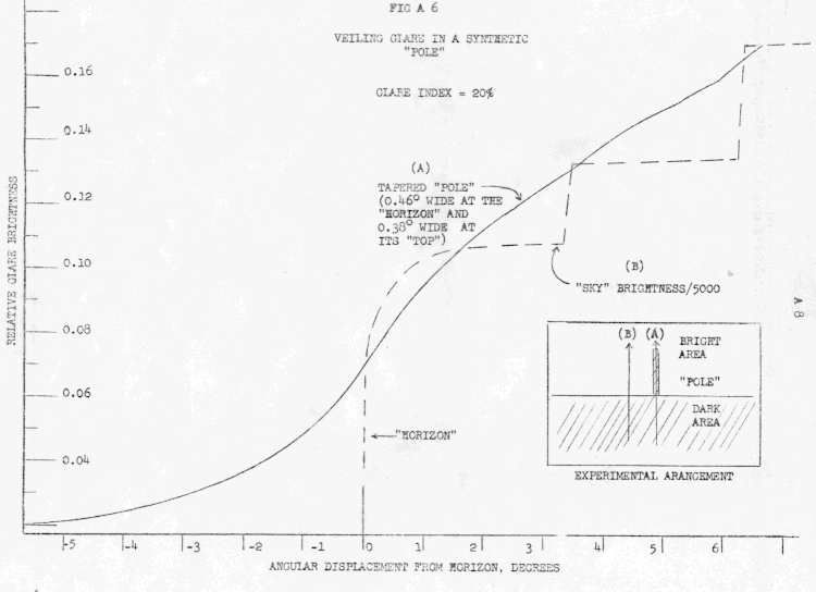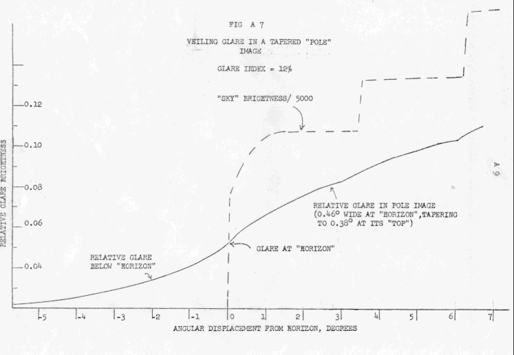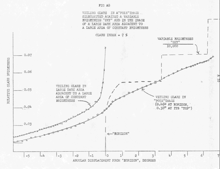Figures A3 and A4 show that the brightness variation of the garage wall is more consistent with guo= 7% than with guo = 12 % or 20 %. Figures A6, A7, A8, A9, A10, A11, A12 & A13 contain glare curves obtained in laboratory simulations of the luminance distribution in photos 1 and 2. 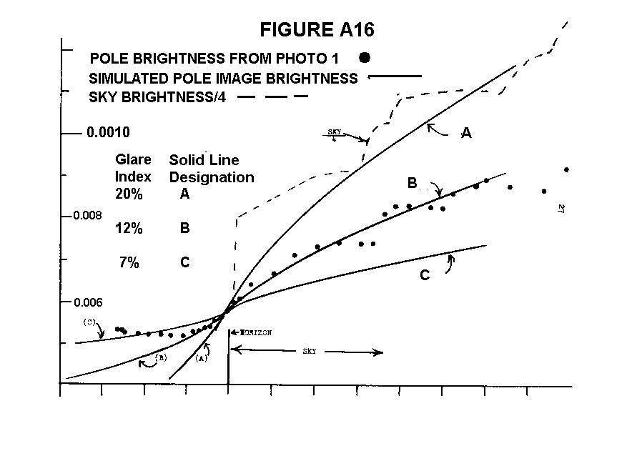Figures A6 A7 A8 illustrate the glare brightness variation along the image of a synthesized "telephone pole" for various values of glare index. These pole simulation curves were used to predict the brightness variation of the image of the pole in photo 1. The predicted variations, illustrated in Fig. A16, were obtained by fitting the laboratory glare curves to the measured Image brightness at the horizon.using the formula Eimage= Bintrinsic + Gimage = Bi + g(x,y) Bs , where Bi, the intrinsic brightness of the object is an adjustable constant (it is constant for a particular graph of brightness versus position on the pole), Bs is the brightness of the sky about 10 degrees above the horizon and g(x,y) is the glare distribution for a given 'sky' luminance distribution and for a given image shape and size as a function of x-y coordinates in the film plane. If y represents angular displacement in the vertical direction, then, along the vertical pole image, Epole image = Bpole + g(y)Bs. The function g(y) for the three glare index values illustrated was, obtained from Figures A6, A7 & A8.
(NOTE: This formulation of the quantitative estimation of veiling glare has a theoretical basis in the observed fact that most of the glare in a image comes from the light sources immediately adjacent to the image, such as from the sky within a few degrees of the UO, for example. In other words, the scattering which produces the glare tends to be a small angle or "forward scattering" phenomenon. The more grease there is on a lens the larger this scattering angle becomes. For typical lenses experiments suggest the angle is a few degrees.)
For example, for guo = 20 %, curve A shown in Fig. A16 is given by Eimage = 0.00151+ g(y)(0.06), where g(y) is the variation of glare with height (y) in Figure A6 (i.e. the graph in Figure A6) and 0.06 is the sky brightness above the pole. To obtain curve 3 in Fig. A16, I have calculated the expected image brightness from Emage = 0.00259 + g(y )(O.06), where g(y) is the variation along the simulated pole in Figure A7. Also in Figure A16 is the expected brightness variation along the pole image when the glare index is 7%. Clearly the best fit to the data (dots) is for 12%.
As can be seen in Fig. A16, all the "theoretical" curves fit the data at the horizon. However, none of them fit the data below the horizon; the photo data indicate a very constant image brightness below 1 degree below the horizon. Thus the data below the horizon are consistent with a glare curve for a glare index even lower than 7%. If the glare index were that low, the increased brightness of the pole image above the horizon in the photo would have to be explained as a combination of glare and intrinsic brightness increase with height along the pole. I have noticed that creosoted poles often become lighter colored near the top as a result of weathering away of the creosote, so it is possible that some of the increased brightness of the pole image with altitude was due to an actual increase in brigtness of the pole, in which case the glare index should be lower than 12%. Unfortunately there is now no way of measuring the actual brightness variations, if any, of the telephone pole.
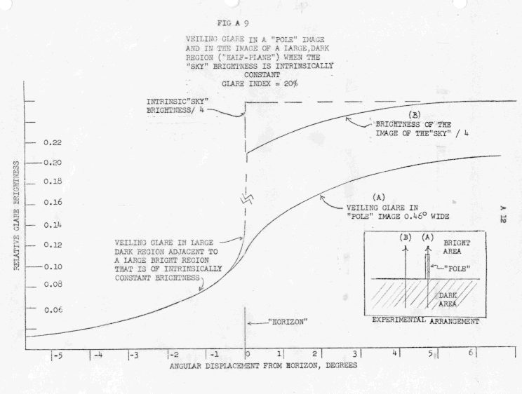
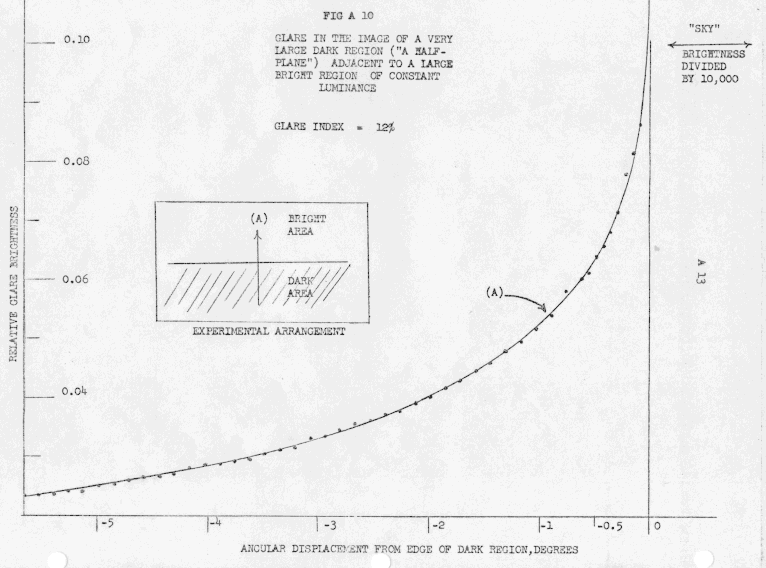
Figures A8, A9 & A10 illustrate the laboratory measurements of VG in a large dark image adjacent to a large bright area, which is an approximate simulation of the garage roof. These curves were used to Calculate the glare curves in Fig. A2.
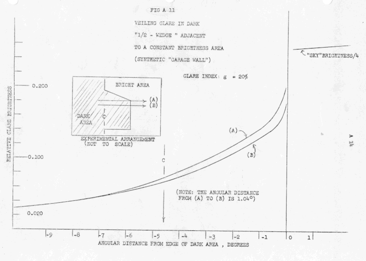
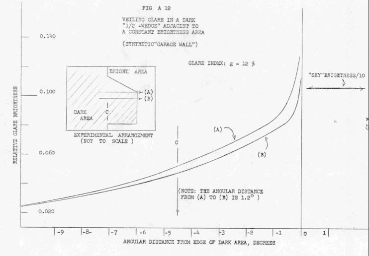
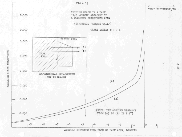
Figures A11, A12, and A13 illustrate the glare variations obtained in laboratory synthesis of the image of the garage when scanned along the rafter ends. These curves labelled "B" in the figures were used to calculate the glare curves illustrated in Figures A3, A4 & A5.
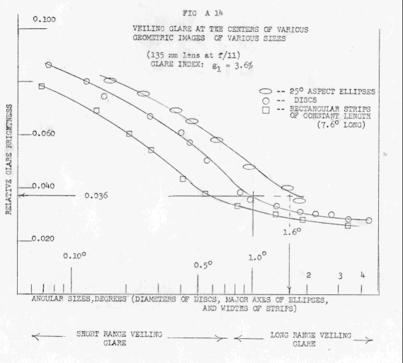
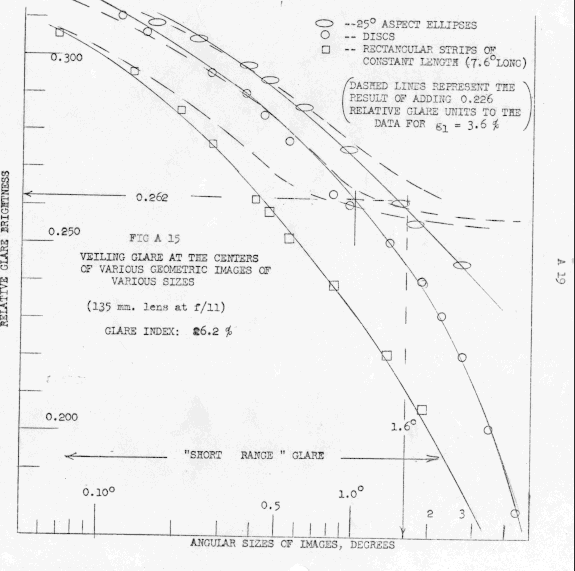
Figures A14 and A15 illustrate the variation of VG with the angular size of an image for various types of simple geometric images silhouetted against a large, constant brightness field. The VG increases as the image size shrinks, although for sizes much smaller than 0.1 degree the VG is expected to remain nearly constant. As an image increases in size the glare shrinks, but it does not go to zero since some light is always scattered. The glare curve can be roughly divided into"short range"and "long range" regions. The short range glare decreases rapidly with increasing image size. When a lens is clean the short range glare is evident for images smaller than a degree in angular extension (depending upon the shape ), as illustrated in Fig. A14. However, when a lens is very dirty the"short range"glare may extend for many degrees, as illustrated in Fig. A15. Also illustrated in Fig. A15 is the observation that an increase in dirt or grease on the lens does not substantially change the functional form of the glare for angular sizes less than 1 degree. Note that the effects of the"short range"glare are also evident in the separation between curves A and B in Figures A11, A12 & A13. Figures A14 and A15 also illustrate the previously mentioned fact that the glare in an ellipse comparable to the image of the bottom of the UO (22 degree aspect ellipse with a major axis length of 1.6 degree) is about the same as in a 1 degree disc.